Datagrok now supports multi-column dimensionality reduction
Dimensionality Reduction capabilities of Datagrok extends the functionality of the Chemical Space and Sequence Space tools, while also providing a way to combine multiple columns and different data types in a single analysis. Each column can be configured with its own encoding function (for example, molecules are first converted to fingerprints), distance metric, weight and other parameters (for example, which fingerprints should be used for molecules). The distances between corresponding values are combined using a weighted aggregation function (Manhattan or Euclidean) to produce a single distance matrix, which is then used for dimensionality reduction.
Usage
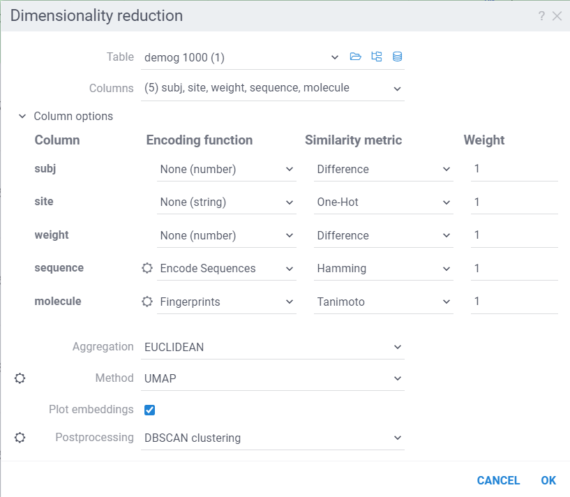
The dialog has the following inputs:
-
Table: The table used for analysis.
-
Columns: List of columns for dimensionality reduction.
-
Column Options: For each chosen column, you can specify what encoding function to use, distance metric, weight, and other parameters.
For example, for biological sequences, you can choose encoding function to convert them to big molecules and then calculate the distance between them using the chemical fingerprint distance, or treat them as sequences and use one of sequence distance functions (Hamming, Levenstain, Needleman-Wunsh or Monomer chemical distance). In case if encoding function can be configured further, you can adjust its parameters using the gear ( ) button next to the encoding function selection. For example, for molecules, you can adjust which fingerprints should be used for encoding.
 -
Aggregation: The function used to combine distances between corresponding values in different columns. The options are:
- Euclidean: The Euclidean distance between two points in Euclidean space is the length of the line segment connecting them.
- Manhattan: The Manhattan distance between two points is the sum of the lengths of the projections of the line segment between the points onto the coordinate axes.
-
Method: The dimensionality reduction method that will be used. The options are:
- UMAP: UMAP is a dimensionality reduction technique that can be used for visualisation similarly to t-SNE, but also for general non-linear dimension reduction.
- t-SNE: t-SNE is a machine learning algorithm for dimensionality reduction developed by Geoffrey Hinton and Laurens van der Maaten. It is a nonlinear dimensionality reduction technique that is particularly well-suited for embedding high-dimensional data into a space of two or three dimensions, which can then be visualized in a scatter plot.
Each method has its own set of parameters that can be accessed through the gear (
) button next to the method selection. For example, for UMAP, you can adjust the number of neighbors,minimum distance,learning rate,epochs,spreadandrandom seed. -
Plot embeddings: If checked, the plot of the embeddings will be shown after the calculation is finished on scatter plot.
-
Postprocessing: The postprocessing function that will be applied to the resulting embeddings. The options are:
- None: No postprocessing will be applied.
- DBSCAN: The DBSCAN algorithm groups together points that are closely packed together (points with many nearby neighbors), marking as outliers points that lie alone in low-density regions (whose nearest neighbors are too far away). The DBSCAN algorithm has two parameters that you can adjust through the gear () button next to the postprocessing selection:
- Epsilon: The maximum distance between two points for them to be considered as in the same neighborhood.
- Minimum points: The number of samples (or total weight) in a neighborhood for a point to be considered as a core point. This includes the point itself.
- Radial Coloring: The radial coloring function will color the points based on their distance from the center of the plot. The color will be calculated as a gradient from the center to the border of the plot.
WebGPU (experimental)
WebGPU is an experimental feature that allows you to use the GPU for calculations in browser. We have implemented the KNN graph generation (with support to all simple and non-trivial distance functions like Needleman-Wunsch, Tanimoto, Monomer chemical distances, etc.) and UMAP algorithms in webGPU, which can be enabled in the dimensionality reduction dialog. This can speed up the calculations significantly, especially for large datasets, up to 100x. This option can be found in the gear (![]() ) button next to the method selection (UMAP).
) button next to the method selection (UMAP).
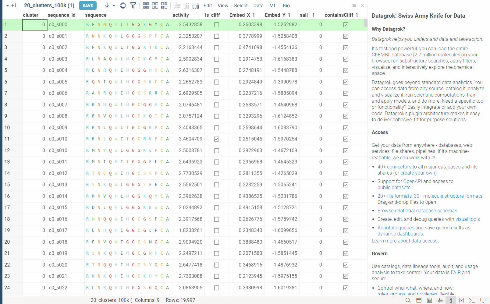
In the example bellow, we perform dimensionality reduction on a dataset with 20_000 protein sequences, which took webGPU implementation 4 seconds to complete (With integrated graphics card, on commodity cards, the speedup is much more). The same calculation on CPU (With our parallelized implementation) took 1 minute and 30 seconds. Commodity graphics cards (like RTX 3060) can perform dimensionality reduction on datasets with 100_000+ rows in under 10 seconds.
Please note, that webGPU is still considered as experimental feature, and for now only works in Chrome or Edge browsers (although it is planned to be supported in Firefox and Safari in the future). If webGPU is not supported in your browser, this checkbox will not appear in the dialog. To make sure that your opperating system gives browser access to correct(faster) GPU, you can check the following:
-
Go to settings and find display settings
-
Go to Graphics settings.
-
In the list of apps, make sure that your browser is set to use high performance GPU.
For more information and details, you can refer to dimensionality reduction help page